This week I was at ICDE’19 where I presented Efficient Synchronization of State-based CRDTs (here’s a link to paper and slides). Following Pedro’s idea, and since the talk is still fresh, this post will be a transcript of it.
Context
In Figure 1, I briefly explain the CRDT acronym. My previous post was just about that.
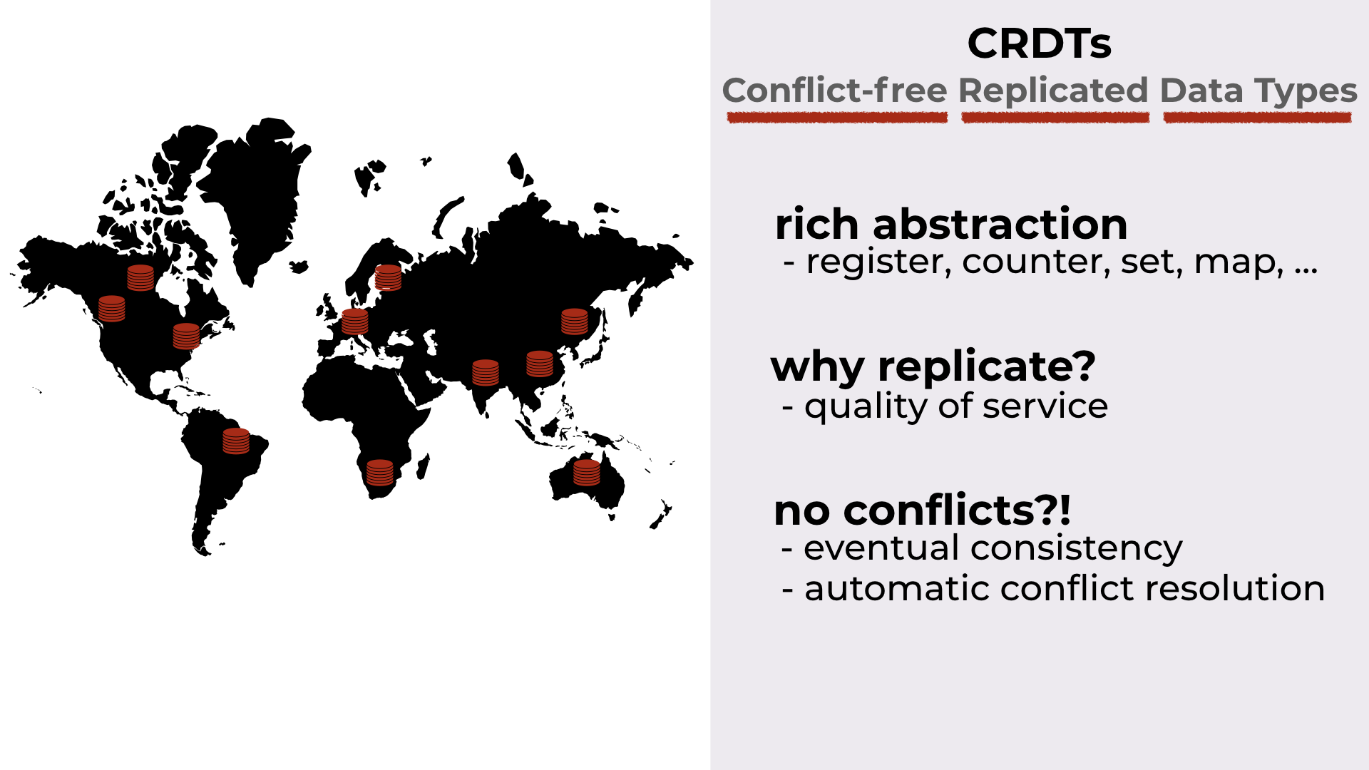
Conflict-free Replicated Data Types.
Outline
CRDT variants: First, we’ll take a look CRDT synchronization models. The main variants are operation-based and state-based. There’s also delta-based, that is a variant of state-based synchronization.
From filter to decomposition; filter; join: In classic delta-based, when a replica receives a delta, it checks whether this delta has something new (the filter), and if it has, the delta is propagated to the peers in the system. We’ll show that this is insufficient, and a more sophisticated approach is necessary: replicas should instead decompose the delta (the decomposition), select the relevant parts (the filter), and then merge them back together (the join), effectively extracting what’s new in the received delta.
A super-realistic example of decomposition; filter; join: Consider a wedding cake. When we decompose it, we get all the layers. Then, we decide that we just want the first and the third layer. In the end, we glue the interesting layers back together.
Decomposition of state-based CRDTs: The filter and join operations are already part of the CRDT framework. We’ll see how they look like in the simplest CRDT (a grow-only set). Then, we’ll introduce the missing part (the decomposition) and the three properties that define “good” decompositions.
And finally, some experimental results before we go.
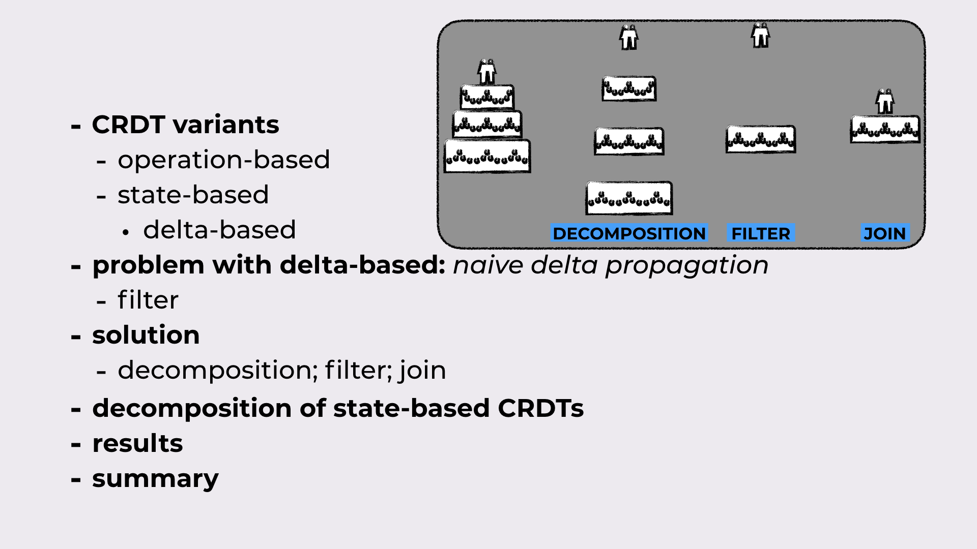
The outline of the talk.
CRDT synchronization models
Two of the main differences between CRDTs synchronization models are:
- the guarantees that the synchronization middleware should provide
- the payload exchanged between replicas upon a new update
Operation-based
In the operation-based model, the middleware should provide exactly-once causal delivery of operations (which can be expensive). The upside: only the update operation (typically small) needs to be sent.
State-based
In the state-based model, messages can be dropped, reordered and duplicated, meaning no expensive middleware is required in state-based. The downside: the full CRDT state needs to be sent when synchronizing replicas.
Delta-state-based
Delta-state-based promises to be the best of both worlds by inheriting the middleware guarantees from state-based (i.e. none), and by exchanging deltas that are typically as small as operations.
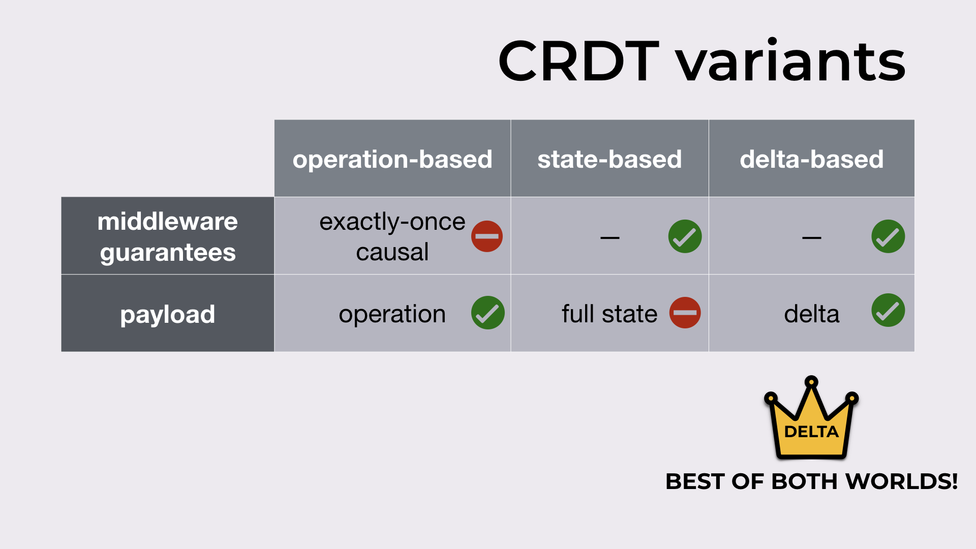
Different CRDT variants (i.e. synchronization models).
But in reality…
There are inefficiencies in the delta-based synchronization model:
In terms of bandwidth (LHS of Figure 4), delta-based can be as expensive as state-based (i.e., effectively sending the full state on every synchronization).
And since large states are being exchanged, trying to compute these deltas results in a substantial CPU overhead, when comparing to state-based (RHS of Figure 4).
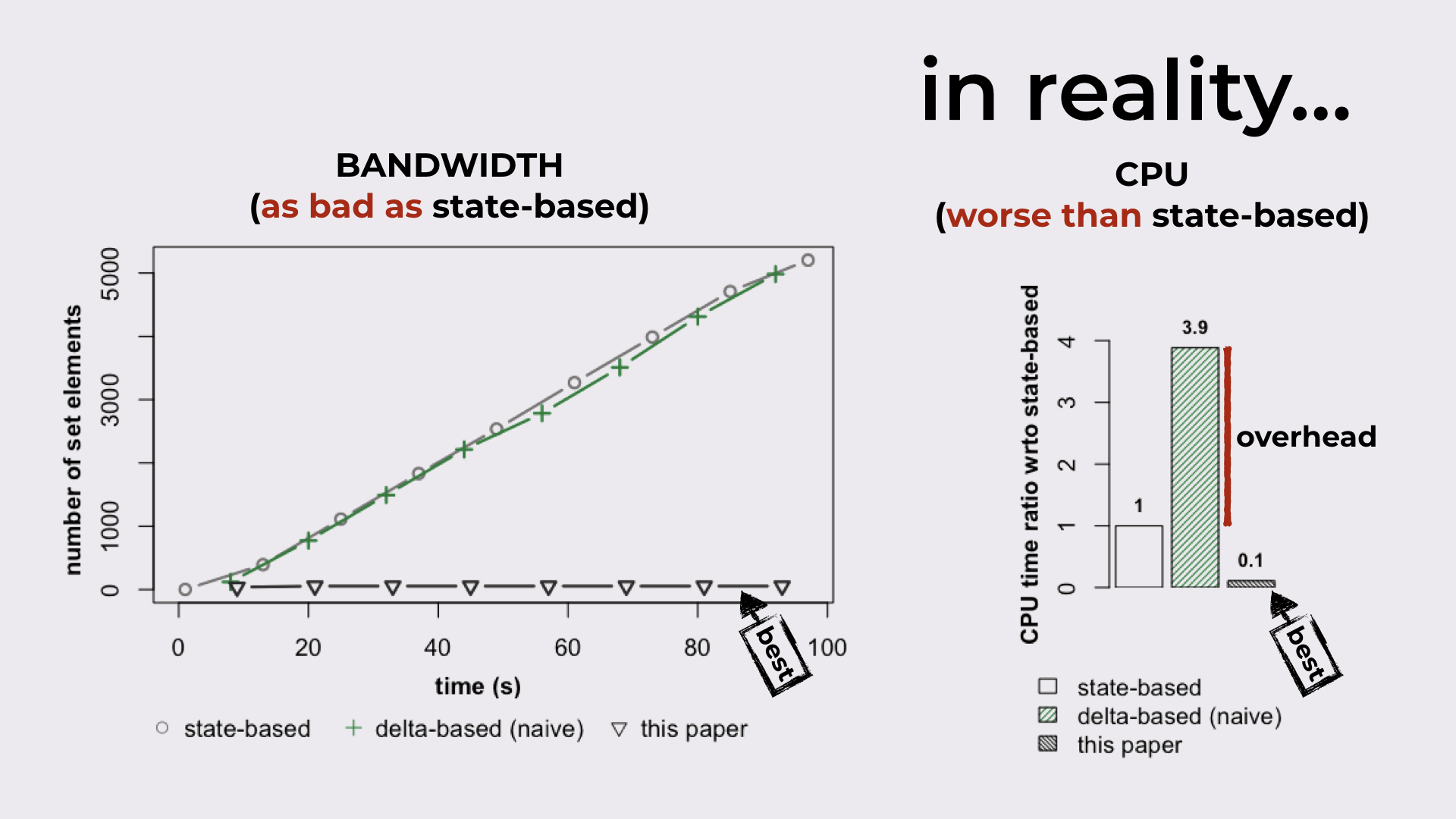
Delta-based can be as bad as state-based in terms of bandwidth, while incurring a substantial CPU overhead.
So, in this paper…
Our main contribution.
State-based CRDTs
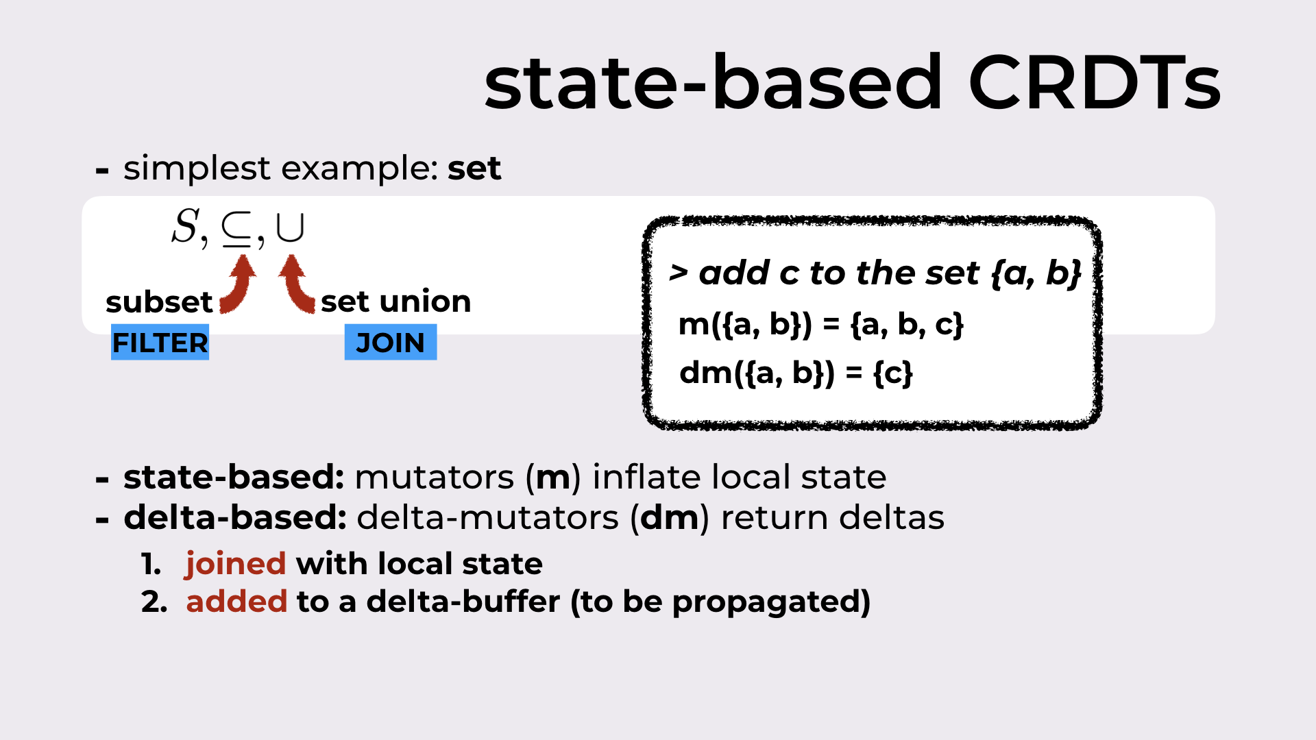
As I promised above, we’ll explore the ideas behind the paper resorting to the simplest CRDT that exists: a set. And from sets, we’ll just need two binary operations: subset and set union.
I mentioned before that all CRDTs have a filter and a join operation. For sets, the filter is the subset, while the join is the set union.
State-based vs Delta-based
State-based CRDTs define functions that allow us to update the CRDT state. These are called mutators.
On the other hand, delta-based CRDTs define delta-mutators that returns deltas. We can think of these deltas as the state difference between the state before the update and the state after.
As an example, if we’re trying to add the element c to a set that contains a and b (i.e., {a, b}), the mutator will return the set {a, b, c}, while the delta-mutator simply returns the delta {c}.
This delta is then:
joined with the local state resorting to join operation (in this case, the set union); after this step, the local state is the same as it would have been if the mutator was used (in our example, we would get {a, b, c})
added to a delta-buffer that contains deltas to be propagated to peers
State-based CRDTs define mutators while delta-based CRDTs define delta-mutators.
Introducing some notation before an example
On the right of our replica, we’ll depict the current CRDT state (an empty set in Figure 7). At the bottom, we’ll have the current list of deltas in the delta-buffer (an empty delta-buffer in Figure 7).
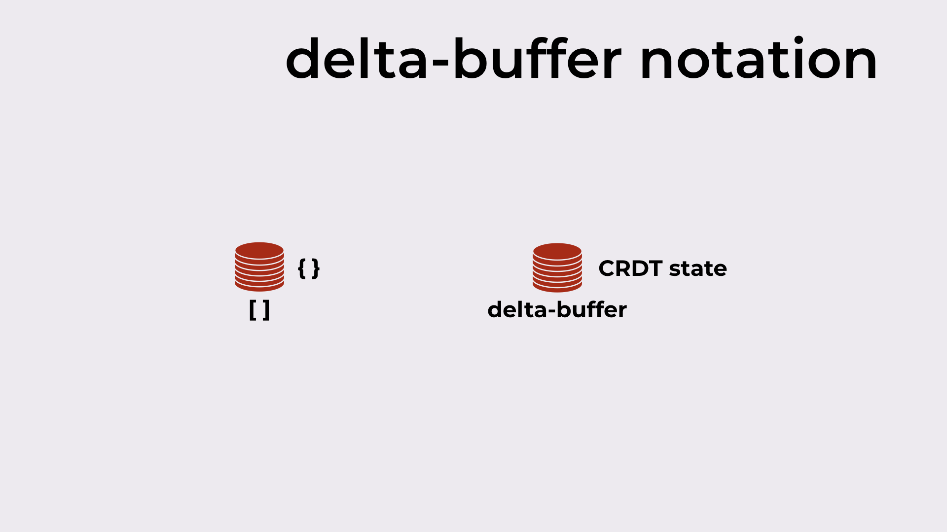
Delta-buffer notation: on the right, the CRDT state; at the bottom, the delta-buffer.
The problem with the classic delta propagation
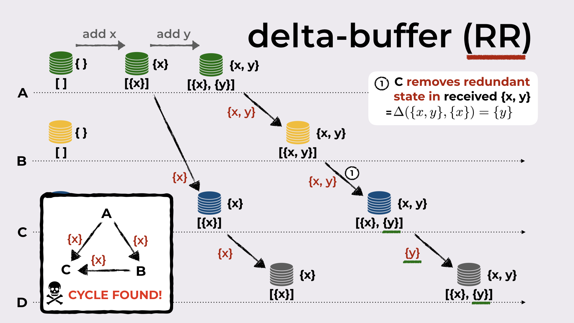
Consider the example in Figure 8 with four replicas, A, B, C, and D. All replicas start with an empty set and an empty delta-buffer.
When A adds the element x to the set, the delta-mutator produces the delta {x}. This delta is joined with the local state (that becomes {x}, since union of { } with {x} is {x}), and it is added to the delta-buffer.
A synchronizes with C by sending the new deltas in the delta-buffer (i.e. just {x}). When C receives this delta, it joins it with the local state and also adds the delta to its delta-buffer, so that this delta can be further propagated.
C syncs with D (the process is similar to the one above).
Now A adds element y to the set. The resulting delta, {y}, is joined with the local state (that becomes {x, y}) and added to the delta-buffer.
A syncs with B by sending the join of all the deltas never sent to B (i.e. {x, y}). B does the standard thing when receiving the delta.
B syncs with C and now we get to the interesting part. Recall that the local state of C before receiving this delta from B is {x}. Although I didn’t mentioned yet in this running example, in the outline of the talk we’ve seen that when a delta is received, a filter occurs: when C receives {x, y}, it checks whether this delta has something new (compared to the local state). And indeed, there is something new (element y)! Since there’s something new, the delta is joined with the local state and added to the delta-buffer.
And finally, C syncs with D by sending the new delta in its delta-buffer (i.e. {x, y}).
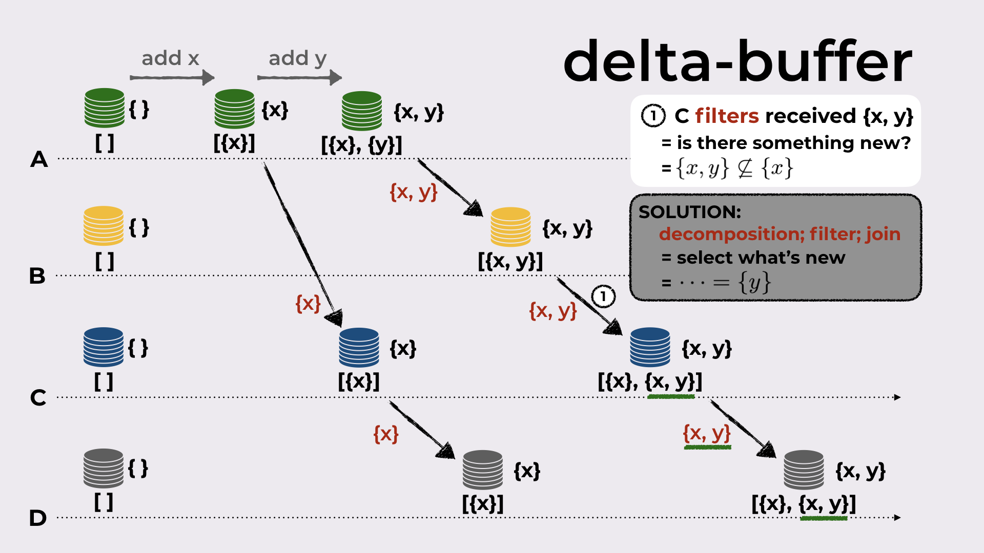
A distributed execution of classic delta-based synchronization showing an inefficiency in delta propagation.
The last step is problematic because C sends {x, y} to D, even though in its previous sync step with D it sent {x}. We would expect that now it would send the new state changes, i.e. only {y}.
This shows that the simple filter done by C when it received {x, y} is not enough! Instead, C must decompose the received delta {x, y}, select/filter the interesting bits, join them back together, and only then, add what results (that should be {y}) to the delta-buffer.
We already know the filter and join operation (at least for sets). Let’s now see how we do the decomposition.
Decomposition of state-based CRDTs
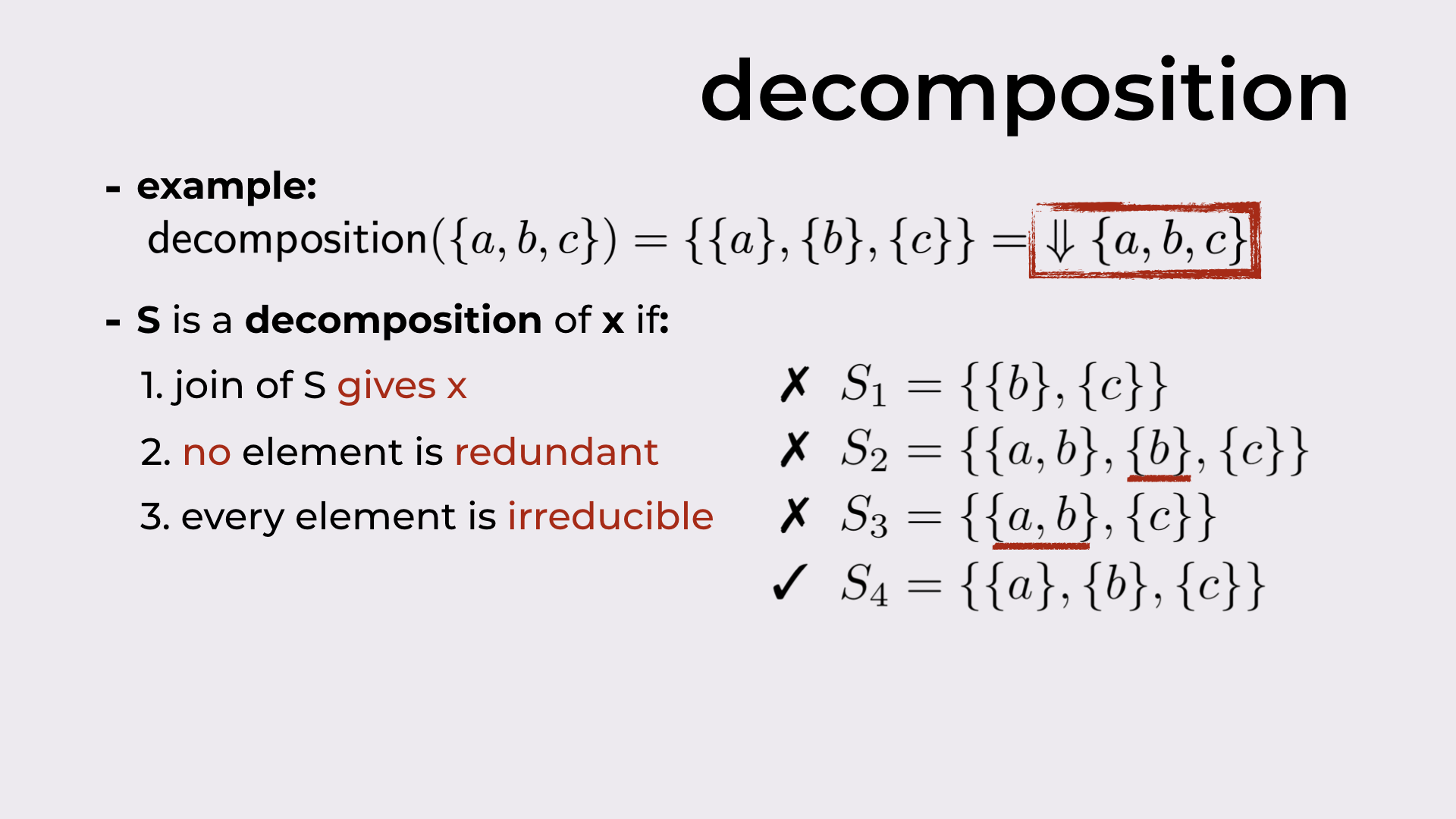
In Figure 9 we have a decomposition example: given the set {a, b, c}, the decomposition of this set should be {{a}, {b}, {c}}1.
In the paper, we define three properties, that when respected, produce “good” decompositions:
- The join everything in the decomposition produces the original element. As an example, {{b}, {c}} is not a good decomposition because its join only produces {b, c}, and not {a, b, c}.
- All elements in the decomposition are needed. {{a, b}, {b}, {c}} is not a good decomposition because {b} is not needed to produce {a, b, c}.
- No element can be further decomposed. {{a, b}, {c}} is not a good decomposition because one of its elements, namely {a, b}, can be further decomposed into {a} and {b}.
Only the decomposition {{a}, {b}, {c}} respects all three properties.
Example decomposition and the three properties of good decompositions.
(In the paper we show that for all states of CRDTs used in practice, a decomposition always exists, and furthermore, this decomposition is unique.)
Introducing the CRDT-difference operation
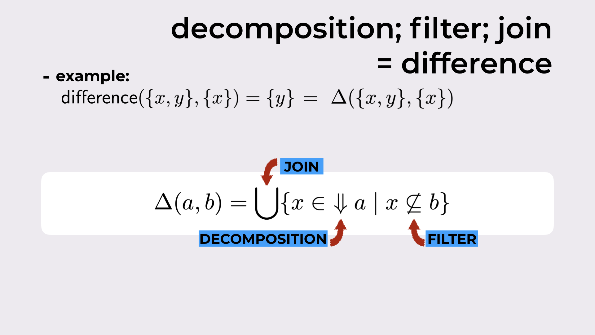
Once we have a decomposition, now we can build a CRDT-difference binary operation.
For sets, this operation boils down to the set difference that can be simply defined as:
$$ a \setminus b = \{ x \in a \mid x \not \in b \}$$
As an example (from Figure 10), the difference between {x, y} and {x} is {y} (i.e. {x, y}$\setminus${x} = {y}).
This operation can be generalized for CRDTs resorting to the decomposition we’ve just introduced. We don’t need to worry much about the formula in Figure 10, but the general idea is the following: for each element x in the decomposition of the first argument (i.e. a), we check whether that x “is needed” in the second argument (i.e. b) resorting to the filter operation; in the end, we join all x that passed the filter, in order to obtain the final CRDT state difference.
A new binary operation for CRDTs.
Going back to our example
Now we’re ready to “fix” our example.
When C receives {x, y} from B, instead of checking if {x, y} has anything new, it computes the difference between the received delta {x, y} and its local state {x}. This returns only the new pieces of information in the received delta, i.e. simply {y}.
The returned {y} is added to the delta-buffer, and now the last sync step is exactly what we expected: only {y} is sent from C to D.
Solving the inefficiency with the difference operation.
Since the replica receiving the delta, removes redundant state in the received delta, we denote this optimization by RR.
Note that this problem only occurred because C received the same piece of information ({x}) from two different replicas: both from A and from B. This means that we have a cycle in the network topology (this will be relevant in the experimental evaluation).
A very simple optimization
In Figure 12 we have depicted another problem in delta propagation: A produced a delta (by adding an element to the set), sent this delta to B, and B sent this delta back to A.
This behavior is undesirable but fortunately it is super simple to fix. Each delta in the delta-buffer should be tagged with its origin (in the example, B would tag {x} with A), and never sent back to the origin in the next sync steps. This optimization is denoted by BP given that replicas should avoid back-propagation of received deltas.
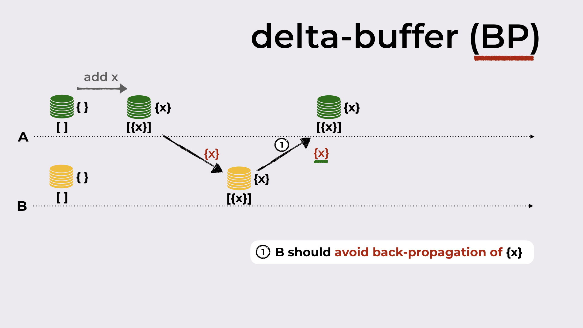
Avoiding back-propagation of deltas.
Evaluation
This post is already becoming super long, so let’s now try to finish it quickly.
As we’ve seen before, cycles in the network topology might result in redundant state being propagated between replicas. With that, in the evaluation we wanted to observe the behavior of the different synchronization models with and without cycles in the topology.
For that, we ran experiments with a tree (acyclic) and a partial-mesh (cyclic). Both these topologies are depicted in Figure 13.
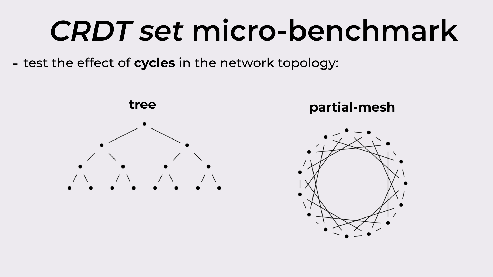
The two network topologies used in the experiments: tree and partial-mesh.
Set micro-benchmark
In Figure 14 we have the bandwidth required by state-based, delta-based, delta-based BP, delta-based RR, and delta-based BP+RR, when synchronizing a replicated set. The results with the tree are on the left, and the results with the partial-mesh are on the right.
- If we look at the first two bars, we can see that vanilla delta-based represents no improvement when compared to state-based, independently of the topology employed.
- The third and fourth bars reveal something interesting: RR is only required when the topology has cycles, since BP alone achieves the best result (BP+RR) in the acyclic topology.
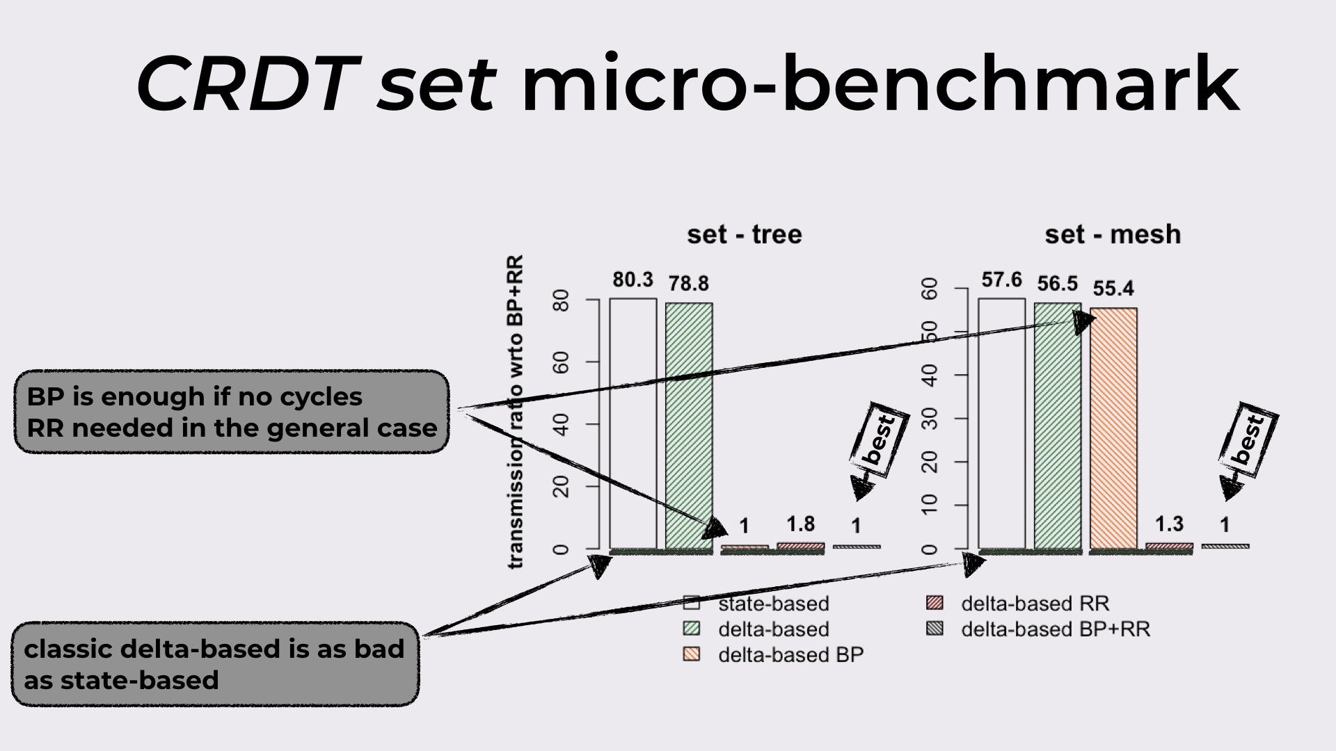
Bandwidth results from the set micro-benchmark.
You may be wondering what’s difficult about that!?!?
For sets, this looks super simple. And I really hope that’s indeed the case, since this was the goal. However, all of this generalizes for any CRDT, as long as we know how to decompose them.
An excerpt from the last appendix in the paper:
In this section we show that for each composition technique there is a corresponding decomposition rule. As the lattice join ⊔ of a composite CRDT is defined in terms of the lattice join of its components [35], decomposition rules of a composite CRDT follow the same idea and resort to the decomposition of its smaller parts.
You can find such rules in Figure 15.
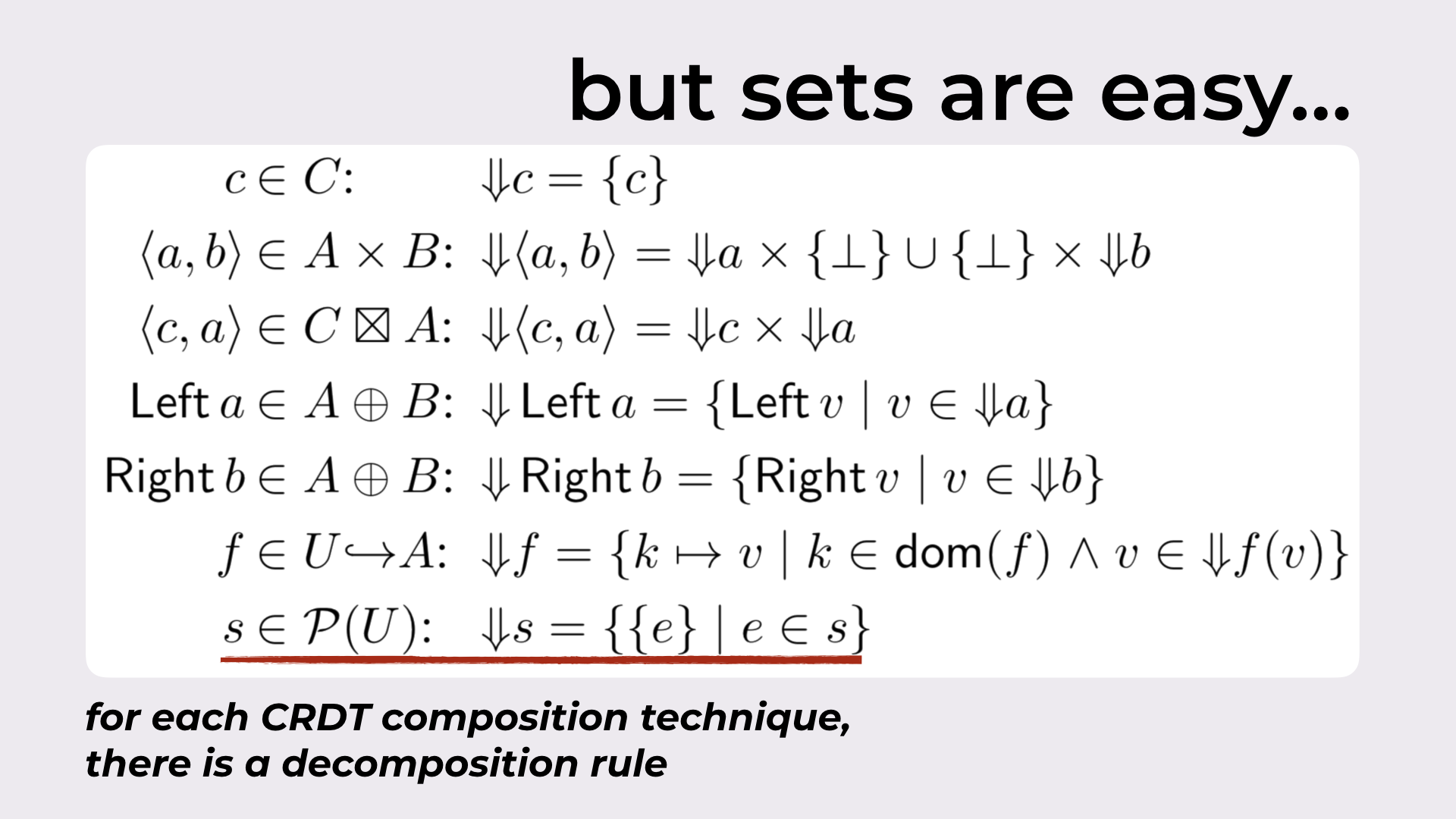
The decomposition rule of each composition technique.
There’s much more in the paper
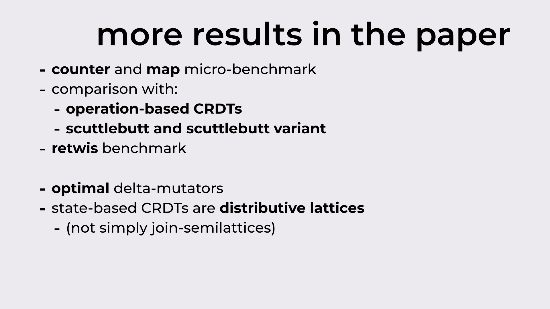
On the experimental side we have other micro-benchmarks (counter and map), comparisons with operation-based CRDTs and two variants of the Scuttlebutt algorithm, and a Retwis benchmark
On the theory side:
- Resorting to the CRDT-difference operation, now we know what optimal delta-mutators should return (optimal in the sense that they return the smallest delta)
- State-based CRDTs are not only join-semilattices, they are lattices, and even more than that, they are distributive lattices!!!
The end
I hope you’ve enjoyed this transcript, and that it didn’t end up being too dense. This paper has also been covered by The Morning Paper.
If any question comes up, don’t hesitate!
- This is basically a set partition with a further restriction (property 3) on the possible elements in the partition. ^